|
| |
 Part A:
Types of Diversions (10 Minutes) Part A:
Types of Diversions (10 Minutes)
The diversions referenced in the tutorial section must be applied to the nodes
themselves. Diversions act to monitor and proportion the amount of flow
contributing to each node and diverting to other nodes.
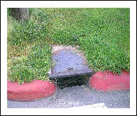
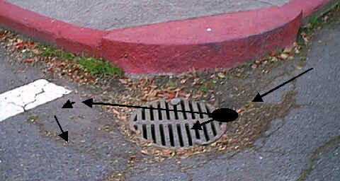
As runoff is collected it proceeds overland and through channelized responses
following a path towards an inlet into the system. At that inlet the water would
follow one or both flow paths. The first path allows the water through grates
and curb openings and into the inlet and drainage systems. The second path will
bypass the inlet with all or a portion of the flow. In the most general case,
all the water enters the inlet. In instances where not all the water can enter
the inlet, the bypassing flow will continue to the next node. This process is
called a “bypass diversion.”

The flow may sometimes pass by the inlet but is curbed by excessively high
street slopes so the flow must settle around the original inlet. This is
referred to as a sag diversion.
Sag diversions provide interesting analysis assuming that all flow up to a
certain depth will enter the inlet and that all flows above that depth will be
diverted such as when the height of the street and the top of curb are taken
into account. As the water pools around the drain inlet the water level
increases adding to the amount of flow entering the inlet. Part of the input
needed to properly analyze a sag diversion are the heights of the street
overtopping locations relative to the rim elevation because the rising water,
once over the street height would flow on to the next inlet. This reaction is
termed a partial sag diversion because it initially allows the water to pool
until a specified depth, then excess water is released as a bypass to the next
inlet once the depth is exceeded. More on this topic is covered in Tutorial 8,
Sag and Sump Inlets.
Critical in flow analysis and flood forecasting, diversions are complex but
worthwhile features to incorporate in your analysis.
Application
Open LessonB.prj from the file menu. In addition, pull out a copy of the Lesson
B Sample System diagram which is page three in the set of diagrams.
Notice that the street sections leading up to inlets 12 and 10 are not marked,
so for the purpose of learning diversions, move on to inlet 13B. A 1% slope
occurs on one side of the inlet and a 2% slope on the other. By sight, this
inlet will be a Sag. Upon further examination, the height required to flow to
the next inlet would be the centerline of the street since the inlets 12B and
10C have a much higher elevation. Instances such as this are an example of a
Sump Inlet. Partial Sag Inlets occur when the flow could go to another inlet on
the same side or could cross the centerline to another inlet.
In order to input this information, click on the S13B node from the main Node
spreadsheet window. Press the Flow Diversion tab that is located in the lower
right corner of the Add/Edit a Node Element Window.
The first step is to find out which inlet would S13B divert to if it would
overflow. Earlier a distinction was made between Sump and Partial Sag by the
ability to overflow beyond the street overtopping height. That statement is
still true but there is a fine line defining the two. Partial Sags only apply
when the height they must top is less than the maximum depth specified. The
software automatically determines if you have a sag or partial sag inlet.
The pull-down menu next to Divert Discharge to Node is for any type of diversion
and must be filled in with a node to continue. In the case of a Sump it
represents the case where extremely high water levels exist and you must decide
where the water would go. Looking at the Lesson B Sample System, the water will
tend to divert to inlet S14C because excess flow will move towards the side with
the 1% slope and cross the centerline closer to S14C.
Click on the Divert Discharge to Node list box and scroll down until you stop on
S14C.
The Flow Diversion Rating Curve Editor works much like the Composite Open
Channel Editor which you worked with in Lesson B. The more time intensive option
is to make your own curve with data points each time that can be loaded and
saved as typical data representative of your project.
The editor uses data points that can be manipulated from the buttons underneath
the table allowing you to Add, Edit, and Delete. Prior to making your own curve,
you must choose which kind of diversion this will become and select it from the
choices.
Your choices are between sag diversions or bypass. The lowest box, Slope of
Inlet Grate allows you to input the slope of the street that leads right up to
and beyond the inlet for bypass diversions only. In most cases, the street slope
is appropriate but in cases where the inlet is recessed it can sometimes be more
accurate to give the slope of the recess rather than street leading to the
inlet.
*Note to the User:
The option to chose Normal Diversion (HGL Based) is misleading. In a previous
version of this software it was used to allow diversions within drainage
systems. This feature will not work with the current version of the software. A
totally new method for calculating internal diversions will appear in future
versions of CS Drainage Studio. The remaining options, Sag and Bypass Diversions
are surface diversions only.
Once the type of diversion is chosen, you can open the data point editor by
clicking on Add.
The Depth box in the Flow Diversion Stage-Discharge editor is made to input the
depth at which the flow in cfs is accumulating at the inlet. The second box is
where the representative flow value can be input.
Input the following data to see the resulting curve.
When completed the Sag Diversion curve should appear in the graph window, but if
it does not simply press the Graph button.
The method for saving your curve is the same as a composite channel. Click on
Save Channel to File and the save window will appear. Any diversion you save
will have the extension *.dv1. Feel free to save this example with any file name
or delete the diversion.
Part B: Bypass Flow Inlets (10 Minutes)
The more common way to obtain your grate capacity curves is from a file using
Get Channel From File which allows you to utilize a pre-made diversion curve
appropriate to your project.
Open the file labeled By2x310. While the names may appear confusing, all the
diversion files provided with the software have been named for ease of use. The
file that you just opened tells you that it is a pre-made bypass diversion for a
drain inlet that has a 2ft. by 3ft. grate opening and has a 1.0% slope across
the inlet.
Slope Examples
When viewing an inlet from a plan and profile print check the inlet profile
first to see whether a drop occurs from street level or if it is flush. If a
drop exists, use that slope as the Slope of the Inlet Grate located in the
bottom right corner. That value can be changed at any time to reflect your data.
*Note to the User:
You should verify whether the inlet capacity curves being used take the recessed
inlet grates into account. If they do the street slope should be used for the
bypass.
If the inlet is flush with the street take the slope of the street leading up to
the inlet. For example, a 2% slope changes to a 1% slope ten feet before the
inlet. Use the 1% slope.
In instances where two slopes are going to a bypass diversion an average of the
two can be used if the grade break occurs close to the grate location within the
flow transition. It may be preferable to assume that the flow transition has
occurred and use the slope at the inlet location. Caution should be used because
most times when two slopes come together the diversion is a sag rather than a
bypass and they do not use slope in their calculations.
Part C: Sag and Sump Inlets (10 Minutes)
For the example Sump diversion at S13B, a sag file would be more appropriate
that a bypass. When you click on Get Channel From File again your options for
sag diversions are much smaller. This is because slopes don’t matter for these
sag diversions where in the case of bypass it can make significant
differences.
The first sag diversion, Rssag, is a sag for a City of Roseville standard type B
inlet. The other files are sag curves for other agencies.
You can make and save diversion curves for specific agency regulations and Civil
Solutions keeps a database of available files which you can add to and download
from our website. Downloadable upgrades for diversions are available at the
website www.civilsolutions.com.
Since LessonB.prj is assumed to be a City of Roseville jurisdiction project,
choose Rssag as the diversion.
Save this node and proceed to the next diversion at either S14C or S14B. Both of
them are bypass and can be modeled with a 2% slope. These inlets diverge to S15B
which can be seen by following the path of the water. The last node with a
diversion is S15B which is a sump and can use the same diversion file at S13B.
Partial Sags are not apparent in the system but they are common in other
residential and commercial developments. If you were to model the partial sag,
use one of the standard sag files available, just as you did for the sump nodes
S13B and S15B. Then determine the maximum height with which the water would
overtop the sag. When the value is less than 1 foot then click on each
individual depth point and click delete.
After doing this multiple times until the largest depth value is the height
required to pass over the sag then you have completed the partial sag
diversion.
Note to the User:
You may have to click on Sag Grate Diversion Type and then press the Graph
button before the diversion will appear in the graph window.
Return node S13B to its correct sump diversion information. This can be done by
reinstating the Rssag file from Get Channel From File.
There is no noticeable change to the Node spreadsheet after inputting all the
diversion types. There will be significant changes, however, when the system is
calculated. Press the full calculation button and the Global Parameters window
appears.
Indicate that you want diversions to be part of the calculations by clicking on
the empty box next to Enable Diversions in the upper right corner. Then press on
the Save Parameters button. Pressing the single iteration button five or six
times after the first calculation should bring the system to convergence.
Diversions will only be computed when diversions are enabled. When this is done
the information will be displayed on the Diversion Summary which is the last tab
on the Results Printout Information spreadsheet.
The information that can be interpreted from the Diversion Summary is that the
diversion did not greatly affect the flow of the system. The added Q values were
low and depth at the inlets did not show more than .36 feet. This depth might be
satisfactory at most locations but would definitely show an encroachment into
the travel way.
Closing Comments
Diversions affect the analysis of a completed system. They can create the need
to change entire systems if bypasses are significant or if the water pools too
high and encroaches into the roadways. Diversion calculations may also show a
need for gallery inlets or supplemental inlets. Diversions are crucial to the
non-visual aspect of CS Drainage and are powerful tools in meeting government
guidelines. For high flow events it may be preferable to disable diversion when
computing the system wiѴh parallel flow since this will force all runoff to
enter the system at the upstream inlet locations.
|